Latency hiding in an empty space
Some time ago, I got a pull request at work for a project that is maintained mainly by me. I am used to reviewing code from my coworkers. So, there was nothing unusual about this pull request, except for one little thing.
I even ranted about this "little" thing on X:
Based on the tweet, you can probably guess who the Co-Authored-By was. But I have to admit, the code itself was pretty clean and easy to review, except that the word deliberate appeared 89 times in the code comments and documentation. This post is not another rant about AI. The problem I am going to write about was not something I could see by reading the code. It only showed up under load, and it took me a couple of days to find.
The essence of this pull request was the HSS server - a new feature integrated into the existing AAA server. Do not worry if you are not in telecom and some terms are not familiar to you. This is really not so important. If you have never heard this abbreviation, just imagine a server that receives incoming network requests, handles them somehow, and returns responses. Something very similar to a CRUD backend server, with just some telecom-specific authentication protocols instead of HTTP, and binary protocol messages instead of JSON.
NOTE
I will try to intentionally use CRUD-like terminology where it is possible in this post to hide unnecessary complexity and avoid requiring prior knowledge of telecom protocols. So, if you work in telecom and know exactly what an HSS is, please forgive me for some simplifications - not everyone is familiar with this terminology and the domain.
After a rough review, I decided to deploy the application with these changes and take a look at its performance. My initial goal was not to solve the C10k problem, but rather to run a relatively medium load and see how the application behaved under it.
I did not expect it to be either super fast or super slow. Just another load test in my life, run to see how the new feature behaves under load, after which I would move on to other tasks.
If my expectations had been fulfilled, this post would never have been written.
Test scenario
My load test was supposed to simulate 250,000 users. Continuing with the CRUD-like terminology, I was going to run the test with the following load profile:
2000Create requests per second2000Update requests per second2000Delete requests per second
Each user starts by sending a Create request to the server. If the request succeeds, the user sends an Update request immediately after receiving the response. Once the last user has successfully completed the Update request, the test returns to the first user and starts sending Delete requests. This creates continuous user-session churn. The sessions are created, updated, and eventually deleted, and the same process repeats throughout the test.
When the application receives an incoming request, it performs some interaction with a MySQL server and then returns a response. In my case, Delete requests did nothing and were implemented as a stub simply because the load-testing tool sent them. So only the database queries related to four thousand Create and Update requests per second reached the database. Each incoming request produces two database queries, one read and one write (or update), so I should expect to see about eight thousand database queries per second.
Obviously, I expected that the database access was going to be the main contributor to the RTT. Because of that, before running the test I was quite curious to see what queries the AI agent had generated and how efficient they were. My expectations were met, but only partially.
First results
I deployed everything I needed for the load test, started the load-testing tool, and... well, see for yourself:

Yes, the 95th and 99th percentile latencies did not look good. Periodically, they reach almost one second!
NOTE
The panel splits the latency by request type. s6a-air and s6a-ulr are the names of the two types of requests that reach the application and produce the database queries. Returning to the CRUD terminology, we can consider them as Create and Update.
The chain of components in my test is simple: application <-> database <-> filesystem <-> disk.
Yes, there are a lot of potential failure points. But for me, the starting point of any investigation in such cases is always pretty clear. When something becomes slow, I think it is usually a good idea to start with the part you control before blaming the components underneath or around it. I know, I know, it is very tempting to blame someone or something else. But believe me, start profiling and investigating from something you can control. You will thank me later.
Of course, MySQL can be misconfigured or used inefficiently, but it is still a mature, production-ready database server that has been developed and tested for decades. With a reasonable configuration and workload, in the right hands, it should behave well. The same is usually applicable to filesystems, at least if you are using something common like ext4 or xfs.
Misbehaving hardware is something that is even harder to believe. Sure, hardware or its firmware can fail or behave unexpectedly under a particular workload, but how often does a performance problem really turn out to be the hardware rather than something wrong in our own code or configuration? If you are not Matthew Dillon, it is probably not so often.
Following my plan to start with the application, I started the investigation.
Know what you measure
Before looking at the application and its database queries, I decided to look at the metric that shows latency. This metric is a Prometheus classic histogram and there is a well-known caveat with them. Their accuracy depends heavily on the chosen buckets. A histogram does not store every observed latency value. Instead, it counts how many observations fall into configured buckets.
When a percentile such as p99 is calculated, Prometheus has to estimate where inside the corresponding bucket that percentile lies. For classic histograms, the histogram_quantile() function does this by assuming that observations are distributed uniformly within the bucket. As the Prometheus documentation says:
When estimating quantiles or fractions of observations in a histogram, or when removing observations from a histogram, PromQL has to apply interpolation within a bucket. In classic histograms, this interpolation happens in a linear fashion. It is based on the assumption that observations are equally distributed within the bucket. In reality, this assumption might be far off.
It could be that this "far off" is exactly my case, so I decided to take a look at the buckets for the metric above:
diameter_if_requests_rtt_milliseconds{type="s6a-ulr", le="30"} 11407669
diameter_if_requests_rtt_milliseconds{type="s6a-ulr", le="50"} 14094452
diameter_if_requests_rtt_milliseconds{type="s6a-ulr", le="75"} 22698461
diameter_if_requests_rtt_milliseconds{type="s6a-ulr", le="100"} 25438069
diameter_if_requests_rtt_milliseconds{type="s6a-ulr", le="1000"} 26110123
diameter_if_requests_rtt_milliseconds{type="s6a-ulr", le="2000"} 26114158
diameter_if_requests_rtt_milliseconds{type="s6a-ulr", le="+Inf"} 26114158
Yes, this is far from ideal. The gap between the 100 and 1000 buckets is quite large. So, a request handled in, let's say, 101 milliseconds is already outside the le="100" bucket, and the next bucket that includes it is le="1000". The problem is that looking at the histogram itself, neither we nor Prometheus can tell whether such a request took 101, 346, or 900 milliseconds because all of them fall into the same (100, 1000] interval. When histogram_quantile() calculates p99, it has to interpolate somewhere inside this very wide range.
As an experiment, we can try to do this interpolation by hand and see what number we will get. The last bucket gives the total number of observations, so we can find which observation p99 is:
26114158 * 0.99 = 25853016
The le="100" bucket holds 25438069 observations, and the le="1000" bucket holds 26110123. Our observation number 25853016 is bigger than the first and smaller than the second, so p99 falls somewhere in the (100, 1000] interval. Now we can repeat something relatively similar to what the histogram_quantile() function would do:
(25853016 - 25438069) / (26110123 - 25438069) = 0.6174

p99 = 100 + 0.6174 * 900 = 656 milliseconds
Using the metric dump above, the interpolation gives 656 milliseconds. Whether these requests took a bit more than 100 milliseconds or were closer to 1000, we still do not know. We see only an interpolation.
NOTE
Yes, 656 milliseconds are not 514 milliseconds shown on the graph. This difference appears because Grafana computes the quantile over a rate window, while the counters we used in the calculation cover the whole run.
The first thing that came to mind was to improve the granularity of the histogram buckets. The dump above already showed that almost all observations were below 100 milliseconds, so I put most of the new boundaries into the range between 100 and 200 milliseconds and dropped the 2000 bucket. After I changed the bucket boundaries and reset the metric, it started to look like this:
diameter_if_requests_rtt_milliseconds{type="s6a-ulr", le="30"} 129560
diameter_if_requests_rtt_milliseconds{type="s6a-ulr", le="50"} 150979
diameter_if_requests_rtt_milliseconds{type="s6a-ulr", le="75"} 260885
diameter_if_requests_rtt_milliseconds{type="s6a-ulr", le="100"} 292176
diameter_if_requests_rtt_milliseconds{type="s6a-ulr", le="125"} 295358
diameter_if_requests_rtt_milliseconds{type="s6a-ulr", le="150"} 297796
diameter_if_requests_rtt_milliseconds{type="s6a-ulr", le="200"} 297946
diameter_if_requests_rtt_milliseconds{type="s6a-ulr", le="250"} 297946
diameter_if_requests_rtt_milliseconds{type="s6a-ulr", le="300"} 297946
diameter_if_requests_rtt_milliseconds{type="s6a-ulr", le="400"} 297946
diameter_if_requests_rtt_milliseconds{type="s6a-ulr", le="500"} 297946
diameter_if_requests_rtt_milliseconds{type="s6a-ulr", le="750"} 297946
diameter_if_requests_rtt_milliseconds{type="s6a-ulr", le="1000"} 297946
diameter_if_requests_rtt_milliseconds{type="s6a-ulr", le="+Inf"} 297946
Now it looks quite different from what I saw before. The time for handling the slowest requests now gets into the (150, 200] interval. I intentionally took the snapshot between the latency spikes because these spikes look like something that should be handled separately.
With more granular buckets, p99 is now somewhere around 121 milliseconds most of the time and Grafana confirms it:

Now it is better. Although as I said, it is still far from ideal. Time to move on and continue the investigation.
Two surprises in the database metrics
After changing the histogram buckets used to measure the latency of handling incoming requests, the p99 latency dropped to about 121 milliseconds most of the time. I could not say this was what I expected. Besides that, there were still occasional p99 latency spikes up to ~990 milliseconds, which bothered me even more.
My next step was to look at the database queries, since they should have the biggest impact on latency. As I wrote at the beginning, with four thousand incoming requests per second reaching the application, I estimated that there would be about eight thousand database queries per second.
It turns out that my estimation was wrong. Here is what the database metrics showed:
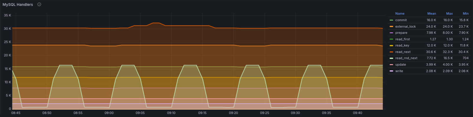
About sixteen thousand commits. This is not what I had roughly estimated during the PR review! It is twice as many as I expected. In addition to the number of database operations being much higher than expected, there are a couple of other suspicious things, like the periodic spikes in the read_rnd_next metric.
That was not so bad in the end. At least now I had concrete questions to answer:
- where the periodic
read_rnd_nextspikes come from - why the database executes roughly twice as many operations as I expected
First of all, I decided to figure out where the read_rnd_next comes from. A growing Handler_read_rnd_next usually means that MySQL is reading rows sequentially, which immediately makes full table scans worth looking for.
NOTE
If you are interested to know more details about this handler, I would advise reading the nice post - A graph a day, keeps the doctor away ! – Full Table Scans by Frédéric Descamps.
After some more digging through the recent changes, I found the source of it. A new metric that had been added executed a SELECT COUNT(...) ... query.
This is a well-known, potentially expensive operation for InnoDB, because it does not maintain an exact number of rows in a table. To calculate COUNT(...), it has to traverse an index and count the rows visible to the current transaction.
In our application, we normally avoid such queries for exactly this reason. If we need this kind of information for a metric or some other purposes, we calculate it once when the application starts and cache the value in memory, periodically bumping it when a counter-related event happens. After I removed this metric query to prove my theory, the read_rnd_next count started to drop.
Counting the queries
Although I dropped the expensive query at the previous step, it did not help a lot with the latency. Yeah, it was to be expected. Even though this query was relatively expensive, it was still periodic, executed only during a metrics scrape. So I continued by revisiting the new database query this PR added. The next potential candidate led me to the answer to why I saw more database queries than I expected.
This candidate was an Ecto query that uses the preload expression. The query itself looks something like this:
query =
  from s in Subscription,
    where: s.imsi == "test",
    preload: [subscription_apns: :apn_profile]
According to the official documentation of this ORM:
Imagine you have a schema Post with a has_many :comments association and you execute the following query:
Repo.all from p in Post, preload: [:comments]The example above will fetch all posts from the database and then do a separate query returning all comments associated with the given posts.
Moreover, the query above uses the nested form, so not only the subscription_apns related to the subscription will be queried, but also the set of related apn_profile records. So, instead of one database query, this ORM expression expands to three database queries like these:
SELECT *
FROM subscriptions
WHERE imsi = 'test';

SELECT *
FROM subscription_apns
WHERE subscription_id IN (...);

SELECT *
FROM apn_profiles
WHERE id IN (...);
One of the ways to avoid these three queries was to use a join. It can be better than three queries, especially if the tables are properly indexed, so I have replaced the previous queries with a query looking something like this:
SELECT
    s.*,
    sa.*,
    p.*
FROM subscriptions AS s
LEFT JOIN subscription_apns AS sa
     ON sa.subscription_id = s.id
LEFT JOIN apn_profiles AS p
     ON p.id = sa.apn_profile_id
WHERE s.imsi = '....';
Despite this query using two JOINs, this should still be quite an efficient query, since the EXPLAIN says that indexes will be used for two tables, and for the last table the primary key will be used:
| table | type | key | rows |
|---|---|---|---|
s |
const |
hss_subscription_imsi_index |
1 |
sa |
ref |
hss_subscription_apn_sub_ctx_index |
1 |
p |
eq_ref |
PRIMARY |
1 |
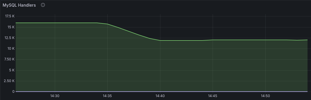
After the query rework, the number of operations dropped to twelve thousand:
In addition, since the number of queries decreased, my expectation was that the latency should also drop. This time, the reality and my expectations matched:
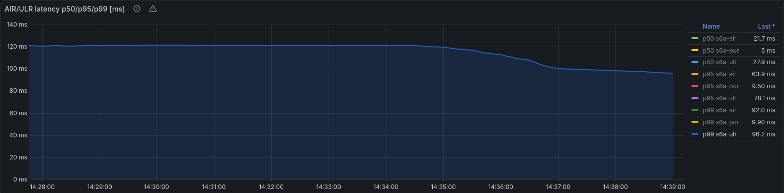
The p99 decreased from ~121 milliseconds to ~96 milliseconds!
Still, the number of queries shown by Grafana was bigger than I expected. Investigating this, I observed that some prepared statements were repeatedly re-opened. We have an application with long-lived connections in a connection pool. In general, it is normal practice to close prepared statements to avoid leaking resources and going over the maximum possible number of them. But in our application we have a finite set of queries. Considering that this small set multiplied by the number of connections will not be bigger than max_prepared_stmt_count, it does not make sense to close prepared statements.
I removed re-creation of prepared statements, and after that I expected to see eight thousand operations. Not so simple!
With this change, the p99 latency now dropped to 30.5 milliseconds, but the Handler_commit metric still showed twelve thousand. It turns out that this status variable does not show the number of COMMIT statements. I have never paid close attention to this status variable and was thinking that it must be equal to the number of transactions, especially since the official documentation does not say anything special:
The number of internal COMMIT statements.
It turns out that this internal COMMIT has a broader meaning than just the number of COMMIT statements. Among other things, the value of this status variable is doubled if the binary log is enabled. It is very clearly visible in the example below:
MySQL [test_hc]> SET SESSION sql_log_bin=0;
MySQL [test_hc]> FLUSH STATUS;
MySQL [test_hc]> INSERT INTO hc_probe (v) VALUES (1);
MySQL [test_hc]> SHOW SESSION STATUS LIKE 'Handler_commit';
+----------------+-------+
| Variable_name  | Value |
+----------------+-------+
| Handler_commit | 1     |
+----------------+-------+

MySQL [test_hc]> SET SESSION sql_log_bin=1;
MySQL [test_hc]> INSERT INTO hc_probe (v) VALUES (1);
MySQL [test_hc]> SHOW SESSION STATUS LIKE 'Handler_commit';
+----------------+-------+
| Variable_name  | Value |
+----------------+-------+
| Handler_commit | 3     |
+----------------+-------+
One inserted row with the binary log off moves the counter by one. The same insert with it on moves it by two! So I cannot fully rely on this metric to know the number of transactions. Twelve thousand is four thousand reads plus four thousand writes, with the writes counted twice because of the binary log. At the same time, Com_stmt_execute shows exactly eight thousand queries. Exactly the number of queries I expected!
The same arithmetic explains the sixteen thousand I started with. The nested preload added two extra queries to each of the two thousand requests per second that used it, and those four thousand extra reads are exactly what disappeared when I replaced it with a join.
The number of queries is finally sorted out, all queries are optimized as much as possible, and the latency is not so scary anymore!
The only thing that still concerns me is the periodic spikes of latency. The most obvious candidate to research is the rest of read_rnd_next. Especially since it also looks periodic.
This was not hard to figure out. I looked around the application code for a periodic job and indeed found one. Disabling it made the last read_rnd_next disappear:

Although it was still not the reason for the latency spikes. They continued...
The last link in the chain
So let's see where we are now. The application behaves as expected and does not produce expensive SQL queries. The load is constant too, and the database does not look overloaded. The database metrics show that all data is read from the InnoDB buffer pool, CPU is not saturated, and there are no visible locks. Still, I could observe periodic spikes of latency. The p99 periodically jumps from 30.5 to about 139 milliseconds. This was concerning for two reasons. The first one, of course, the existence of these spikes. But my main concern was that I did not understand what was going on!
Before I reworked the queries, the latency reached 990 milliseconds. Now it reaches about 139 milliseconds. Some kind of periodic slowdown exists. Nothing underneath the application changed between these two measurements. Only the number of queries changed. When the number of database queries was bigger, I could observe that the queue of the connection pool grew during the whole slowdown. With fewer queries there is more room in the connection pool, so the same slowdown builds a much smaller queue. The optimization of the database queries did not remove the cause of these spikes, but only made the application less sensitive to them.
Nothing to do, need to dig deeper.
OK, so the application works well and the database server behaves normally. What can it be? The disk? Let's see.
Looking at the database and the node metrics, I noted another interesting thing. The rate of fsync operations starts to go down exactly at the time of these latency spikes:
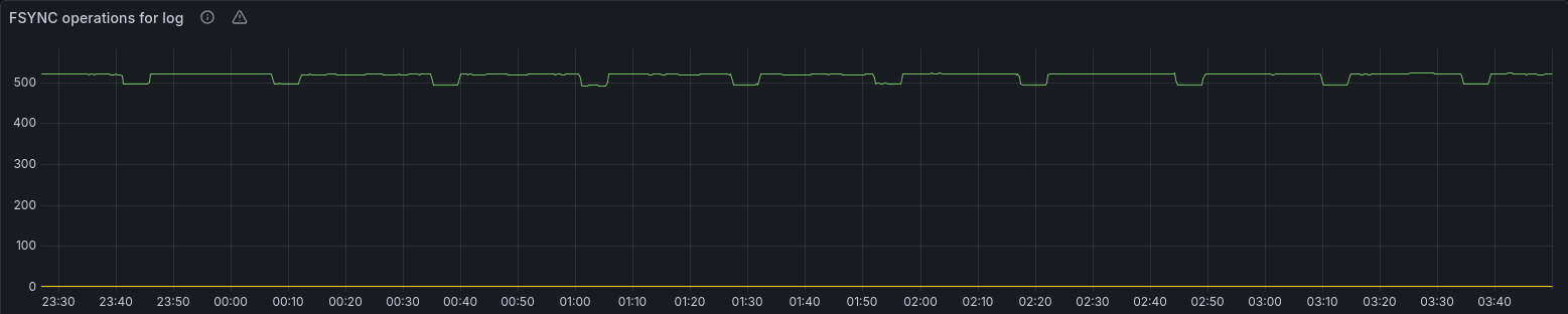
What is it? The MySQL server is blocked by something and starts to execute fewer fsync operations? Or fsync operations themselves start to be slower and because of this the MySQL server waits for them, so the next ones have to queue? Or both? It would be interesting to take a look at the flush rate from the device perspective. I can get this information using the following metric:
rate(node_disk_flush_requests_time_seconds_total{....}[$Interval])
  / rate(node_disk_flush_requests_total{....}[$Interval]) * 1000
It shows that something is definitely happening with the device periodically, and it happens exactly when the latency spikes:
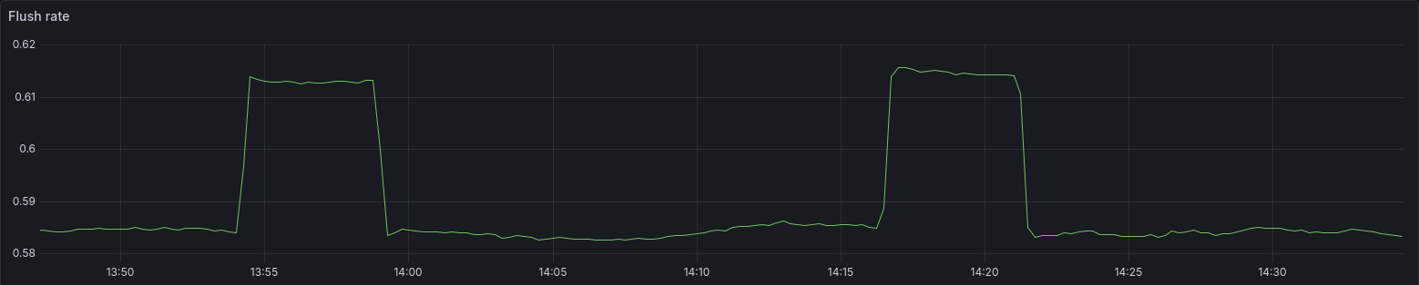
This kind of answers the question I asked above. The rate of fsync operations goes down and at the same time the time per flush goes up. If it were something related only to the MySQL server, like, if it executed fewer flushes because of some internal reasons, the device should have less work to do. And in this case I should see the time per flush stays flat or even drop. But it is not my case. So, it seems that the device becomes slower, and the lower rate of fsync operations is just a consequence of that.
NOTE
The size of this change on the panel above does not mean much. It is an average over a 5 minute window where the slow flushes are mixed together with the normal ones.
I decided to stop the load test and run the fio util with a similar load profile to see what would happen. Yes, it can sound contradictory to what I said before, that most likely there is something wrong with software rather than with hardware. But in this case, MySQL is not the software that I developed, and running a short fio test is certainly easier than debugging potential data-flush issues in a MySQL server. Moreover, it makes the test independent of my application and MySQL.
Yes, it might be that the load profile I scripted for fio does not repeat exactly what MySQL does with the disk, but it should do something relatively similar:
| job | models | writes | durability | matching setting |
|---|---|---|---|---|
redo |
InnoDB redo log | 8k buffered, 700 iops |
fsync per write |
innodb_flush_log_at_trx_commit=1 |
binlog |
Binary log | 4k buffered, 700 iops |
fdatasync per write |
sync_binlog=1 |
pages |
InnoDB page flushes | 16k random, direct=1, 250 iops |
no fsync |
innodb_io_capacity=200 |
It turns out it was the right decision!
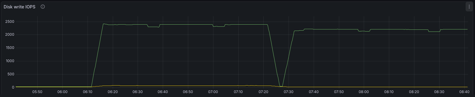
As we can see on the graph above, the test with fio (right side) dips in exactly the same way as the test with MySQL (left side). fio sends writes at a fixed rate that I configured, and there is no application above it that could decide to do less work because of queuing or something like that. So if the write rate of fio drops, the reason is somewhere below it. What can it be? The filesystem or the device itself.
Time to look at the concrete numbers. Let's see what one write plus one fsync actually costs:
redo: (groupid=0, jobs=1): err= 0: pid=2752317
  write: IOPS=433, BW=3472KiB/s (3555kB/s)(11.9GiB/3600001msec)
    clat (usec): min=3, max=369, avg=10.02, stdev= 5.78
    ...
  fsync/fdatasync/sync_file_range:
    sync (usec): min=564, max=30434, avg=2291.21, stdev=869.63
The write itself takes about 10 microseconds. The fsync after it takes 2291 microseconds on average, and the range across the run goes from 564 to 30434 microseconds. Writing the data is about 229 times cheaper than making it durable.
The redo job asked for 700 operations per second and got 434:
iops : min= 84, max= 669, avg=433.99, stdev=48.24, samples=7199
One operation is one write plus one fsync, so 10 microseconds plus 2291, and the highest possible rate is 1 / 2.301ms, which is 434.6 per second. The run reports an average of 433.99. The device delivered exactly what its fsync latency allows and nothing more. It looks like this job is not limited by how much data the drive can write, but rather how long the drive takes to answer a flush.
At the same time, the device was not even fully busy:
Disk stats (read/write):
  nvme0n1: ios=1552/10654162, merge=1/1621885, ticks=384/6266480,
           in_queue=10522664, util=70.82%
70.82% utilization over a full hour, and in_queue divided by the time of the run gives an average queue depth of 2.9. The device had spare capacity the whole time. All three jobs were simply waiting.
The iops of all three fio jobs show the same pattern:
| job | sync call | min iops | avg iops | max iops |
|---|---|---|---|---|
redo |
fsync |
84 | 434 | 669 |
binlog |
fdatasync |
164 | 700 | 850 |
pages |
none | 248 | 250 | 252 |
The pages job never flushes, and in the whole hour it never dropped below 248 operations per second against its target of 250. So yes, the periodic slowdown does not touch the writes, but only the flushes.
But the device is not the only thing involved in a flush. Between fio and the drive, there is still the filesystem, ext4 in my case. And on ext4, an fsync not only flushes the written data to the drive, but it also forces the journal to commit.
So I decided to trace the journal. ext4 emits a tracepoint for every committed transaction, and jbd2_run_stats shows where the time of each one went. I enabled tracing like this:
cd /sys/kernel/debug/tracing

echo 1 | sudo tee events/jbd2/jbd2_run_stats/enable

sudo cat trace_pipe | while read -r l; do echo "$(date +%H:%M:%S) $l"; done
I started to wait for the next spike. I did not have to wait long. The next spike appeared around 20:57:45. I stopped the tracing and selected the records around this time:
20:57:20  jbd2_run_stats: wait 0 request_delay 0 running 5000 locked 0 flushing 0 logging 4  blocks_logged 39
20:57:25  jbd2_run_stats: wait 0 request_delay 0 running 4992 locked 0 flushing 0 logging 3  blocks_logged 30
20:57:30  jbd2_run_stats: wait 0 request_delay 0 running 5000 locked 0 flushing 0 logging 3  blocks_logged 25
20:57:35  jbd2_run_stats: wait 0 request_delay 0 running 4995 locked 0 flushing 0 logging 13 blocks_logged 26
20:57:40  jbd2_run_stats: wait 0 request_delay 0 running 5000 locked 0 flushing 0 logging 10 blocks_logged 29
20:57:45  jbd2_run_stats: wait 0 request_delay 0 running 4987 locked 0 flushing 0 logging 15 blocks_logged 26
20:57:50  jbd2_run_stats: wait 0 request_delay 0 running 5000 locked 0 flushing 0 logging 9  blocks_logged 28
20:57:55  jbd2_run_stats: wait 0 request_delay 0 running 4983 locked 0 flushing 0 logging 3  blocks_logged 21
Let's start from the field for which the changes are the most visible - logging. This is the phase where the journal writes its blocks and waits for the device to confirm the commit. Usually it takes about 3 milliseconds, but during the latency spikes it visibly grows. What is really interesting is that the blocks_logged does not grow. So the journal did not write more data than usual. Every phase where it could be blocked by something of its own is zero. It just waits longer for the data to be flushed, exactly like MySQL does.
So the journal does not look like the cause. It slows down for the same reason my fsync does. So what is it in the end? The disk? Really? Let's at least see what disk it is:
sudo smartctl -i /dev/nvme0 | grep 'Model Number'
Model Number:                       KXG60ZNV1T02 TOSHIBA
Well... this is not an enterprise SSD. fsync on it does not have the best performance, and OK, it is expected from a consumer SSD. But what happens with it periodically, I do not know. Something wrong in the firmware? Some housekeeping or garbage collection inside the drive? I really do not know. I was close to giving up and running the same test on another node with different disks, but...
What it actually was
Trying to accept this failure, I decided to look at something I had never looked at before:
sudo fstrim -v /
/: 784.9 GiB (842729443328 bytes) trimmed
The drive is 1 TB and only about 109 GiB of it was in use. The command discarded 784.9 GiB in one go, which means none of that space had ever been discarded before. To be honest, I cannot say I expected any significant changes executing this "innocent" command, but here is what I saw after another fio run:
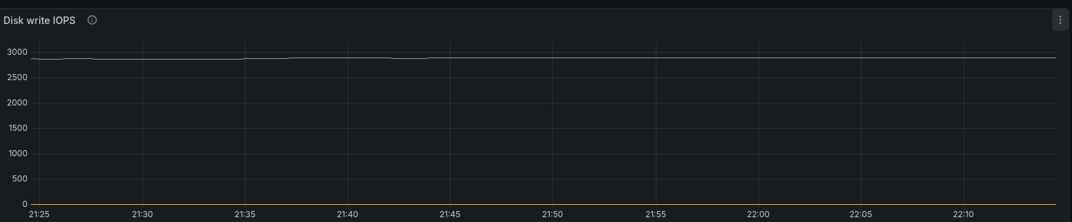
The panel covers fifty minutes of that run, and the periodic dips are gone! I could not believe my eyes. I ran the application test and:
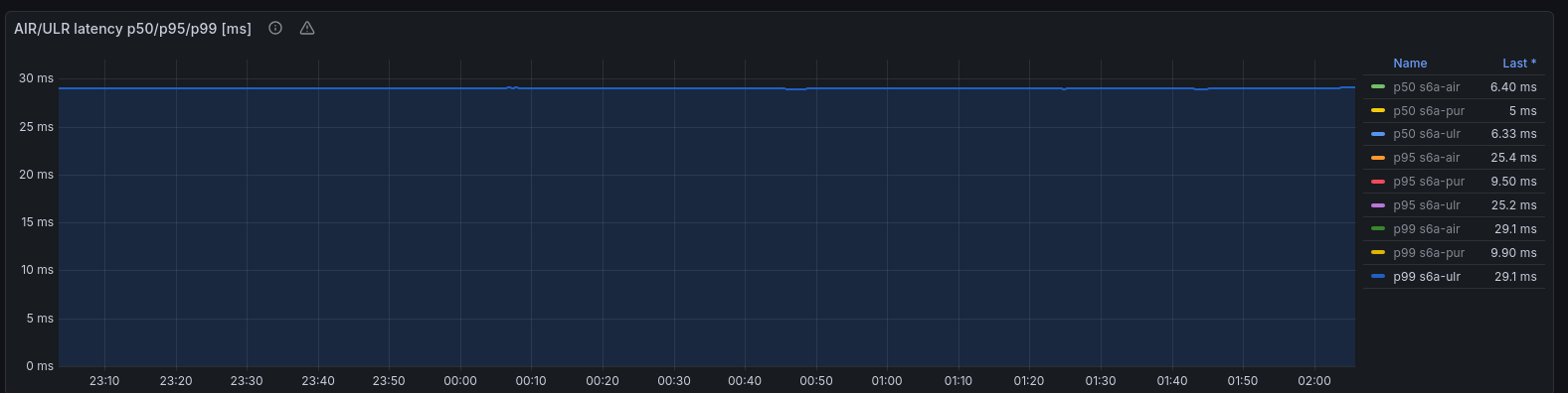
No latency spikes anymore! Three hours of the same load profile, and p99 holds at 29.1 milliseconds, while the spikes used to come every twenty minutes or so.
I cannot say for sure why it helped to eliminate the periodic stalls, so what I have at this point is only a theory rather than something I can prove. What I know is that an SSD cannot overwrite in place. It writes new data somewhere else and marks the old copy invalid, and later it reclaims those blocks. As far as I know, it finds out that a block is no longer needed only when the host writes something new there or sends a discard.
My theory is that the drive simply did not know that all this space was free. It had been rewritten many times, so from its point of view almost every block still held live data. Every time it needed a free block, it had to copy that data somewhere else and only then erase. All this copying happens in the flash, and a flush has to reach the flash too, so it waits until the drive is done. A write without a flush does not wait, because the drive answers it from its own memory.
Of course, the flush itself did not become faster. It costs the same as before the trim, and this was expected. Nothing here changes how long this drive needs to make data durable. What went away is the drive becoming periodically slow. It may be that the drive was always doing this housekeeping. The trim should not stop this process of course, but it seems it made each round cheap enough that nothing above can notice it.
You know the feeling I had looking at the last graph, right 😊?
As I said, this is still just my theory, based on what I roughly know about fstrim and how SSDs manage their blocks. If you have something to add, or want to point out where I am wrong, please feel free to reach me on X. I would really appreciate it.
Conclusion
Well, what can I say in conclusion... Reworking the queries brought significant improvements, but the last part of the story was not in my code. The test revealed two more things, and both are about my test environment. The free space on this drive had never been discarded, and a single fstrim was enough to fix that. The other one is what fsync costs on a consumer SSD.
It is probably the right time to quote Peter Zaitsev from his post - Why Consumer SSD Reviews are Useless for Database Performance Use Case
If you’re reading consumer SSD reviews and using them to estimate SSD performance under database workloads, you’d better stop. Databases are not your typical consumer applications and they do not use IO in the same way.
The KXG60ZNV1T02 may look like a perfectly capable SSD if we judge it by the usual consumer metrics like sequential throughput, random IOPS, and so on. But none of these numbers say anything about how the drive behaves when an application keeps asking it to make data durable.
A database asks for fsync all the time. Every Create and Update request in my test ended up waiting for one. On this drive, a write costs about 10 microseconds, and making that write durable costs almost 229 times more. A drive with power loss protection usually answers in tens of microseconds, because it can promise durability from its own memory. Of course, none of this means this device is "broken"; it was just built for different tasks.
In the end, I would like to briefly revisit a few practical lessons from this investigation. At least to repeat them for myself and keep them in mind:
-
Be careful with histogram buckets. A histogram is only as useful as the bucket boundaries chosen for it. Before I changed anything, my
p99came from a bucket that covered everything between100and1000milliseconds. If most observations fall into one or two buckets, percentiles calculated from that histogram can be misleading or simply too rough to diagnose the problem. -
Do not immediately blame the hardware. In my concrete case, the hardware did play a significant role. Despite that, it is still usually much easier to re-check something that you can control. Revisiting the application side alone brought the improvements for
p99from121to30.5milliseconds. -
How much a slow dependency hurts depends on how much room you have above your load. In my case, the same disk produced spikes of
990milliseconds when the database was close to its capacity and about139when it was not. -
Check that unused blocks are actually being discarded. On my node
fstrim.timerwas reported as active and the drive had still never been trimmed. Why it never fired is something I still have to debug, but this is probably a story for another post.
And this is where I finish my little story about a couple of days of debugging.
Do not give up and have fun debugging!